Exploration 5.9.2.
In this exploration, we want to examine whether curvature depends on the particular parameterization used or just the location on the curve at which the measurement is taken. With all of the specific values given in the problem, try to get as close as possible even if you can’t get right on a particular value.
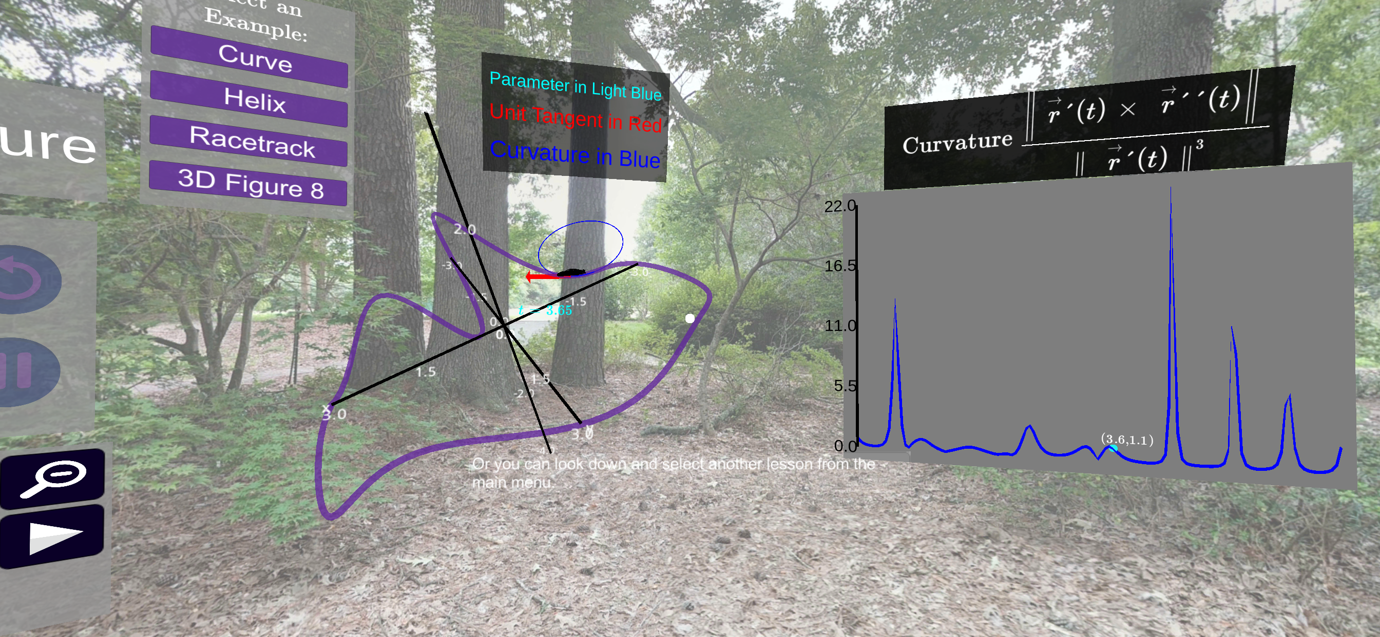
To get started, make sure your headset and controller is set up with the CalcVR app. Start the CalcVR app go to the Vector Valued Functions set of lessons. Start the Vector Valued Function Demo and put your phone in your headset. Once the Demo loads, a 3D graph of a curve in space should generate in front of you with a plot of related scalar quantities to the right. The function input panel will show up on the left of the 3D plot and an option selector panel will show up below the 3D plot.
You should use the option selector panel to turn off all vectors except for the position vector. On the function input panel, select the Preloaded Inputs button and scroll until you reach Exploration 1. Click the Display button to load these functions. If a new plot does not automatically generate, then click on the Plot Graph button to the bottom right of the function input panel. You can use the slider at the top of the option selector panel to move the car to different spots on the curve. Note that as you change the car’s location, the \(t\)-value of the location is updated and the corresponding plot is highlighted on the 2D plot to the right.
(a)
Sketch the graph of curvature and note the scale on both axes. Be sure to use the scale on the left of the plot (in blue). Additionally, you should plot and label the points that correspond to \(t\)-values of 1.5, 2.6, 4.4, and 5.2. Be sure to note the position of these locations on both the 3D and 2D plots. We will be comparing these same locations across different vector valued functions.
(b)
Select the Preloaded Inputs button at the bottom of the Function Input Panel. Scroll to the Exploration 2 functions and select the Display button. The same curve as was used earlier should be rendered but the parameterization used moves through these points twice as fast in terms of t. Note that this means half of the range of t. You should use the Option Selector Panel to turn off all vectors except for the position vector.
Draw the graph of curvature for the parameterization of Exploration 2 and be sure to note the scale for both the vertical and horizontal axes. Additionally, you should plot and label the points that correspond to \(t\)-values of 0.75, 1.3, 2.2, and 2.6. Be sure to note the position of these locations on both the 3D and 2D plots.
(c)
Write a paragraph that answers the following questions: Is the shape of the curvature graph different? What changed for the values of the curvature? What changed on the horizontal scale?
(d)
Select the Preloaded Inputs button at the bottom of the Function Input Panel. Scroll to the Exploration 3 functions and select the Display button. The same curve as was used earlier should be rendered but the parameterization used moves through these points exponentially fast. You should use the Option Selector Panel to turn off all vectors except for the position vector.
Draw the graph of curvature for the parameterization of Exploration 3 and be sure to note the scale for both the vertical and horizontal axes. Additionally, you should plot and label the points that correspond to \(t\)-values of 0.69, 1.13, 1.58, 1.74, and 1.9. Be sure to note the position of these locations on both the 3D and 2D plots.
(e)
Write a paragraph that answers the following questions: Is the shape of the curvature graph different? What changed for the values of the curvature? What changed on the horizontal scale?
(f)
You may be tempted to say that curvature is a property of the driver based on your graph for Exploration 3, but remember that the horizontal axis is based on the parameter not the location on the curve. Using the additional values you labeled on your plots, verify that the same locations on the curve have the same values for the curvature measurement.