CalcVR Supplemental Materials

Section 6.7 Directional Derivatives

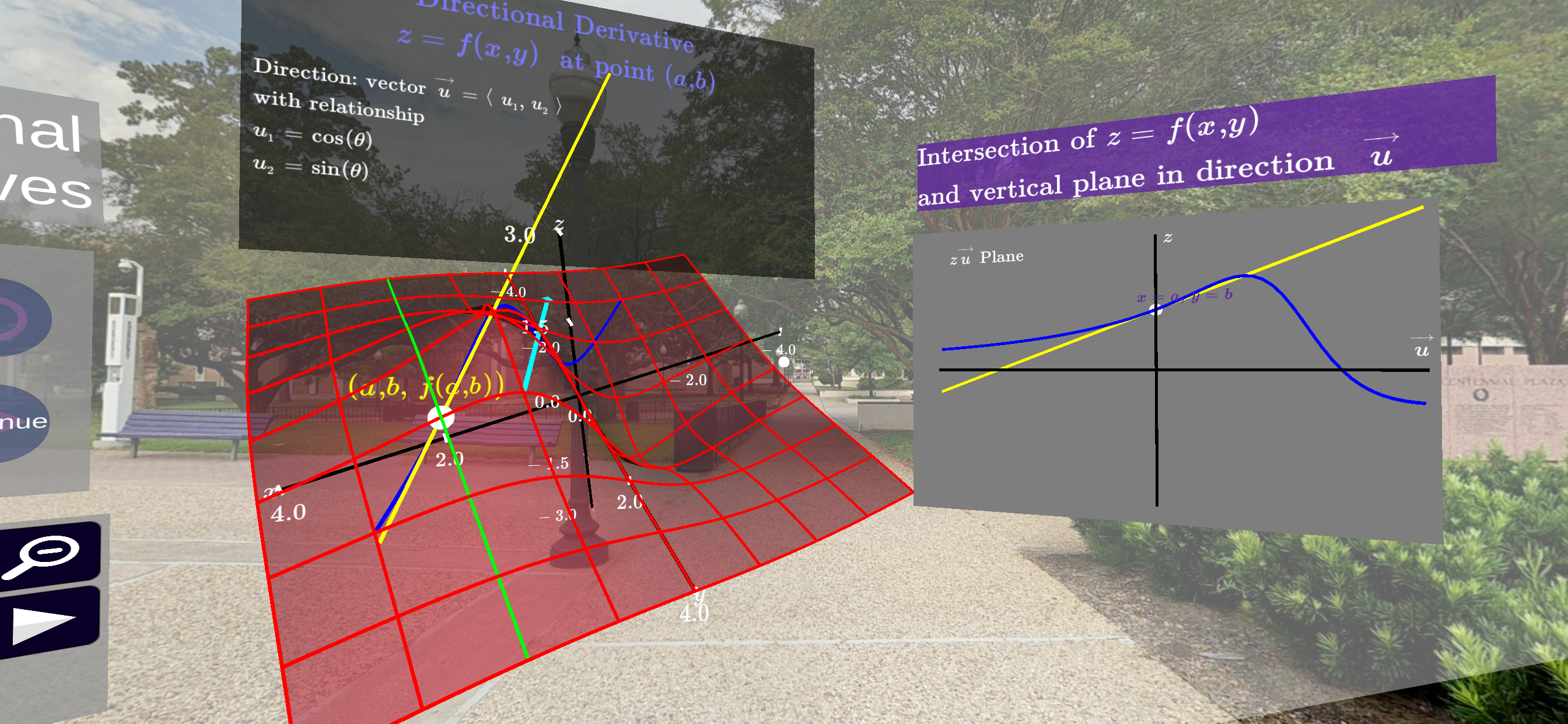
Figure 6.7.1. A screenshot from the lesson on directional derivatives of multivariable functions.
In the CalcVR lesson, the geometric ideas presented in the lesson on partial derivatives are generalized to define the directional derivatives. In particular, the linear combinations of partial derivatives are used to compute the rate of change in a particular direction. Several examples are shown with both partial derivatives highlighted along with the directional derivative in several different directions. We have also examined the concept of derivatives of paths (or parametric equations) in Section 5.2. Both of these concepts involve a rate of change and thus should be connected.

Subsection 6.7.1 Connection to Vector Valued Functions

Example 6.7.2.

Consider the example of the multivariable function
\begin{equation} f(x,y) = x^2/4 - y^2/9\text{.}\tag{6.7.1} \end{equation}
First let’s find the directional derivative at \((2,3)\) in the direction of \(\mathbf{v} = \langle -1, -2 \rangle \text{.}\) The partial derivative of \(f\) with respect to \(x\) and \(y\) are simple enough to compute
\begin{equation*} f_x(x,y) = \frac{x}{2} \qquad \text{and} \quad f_y(x,y) = -\frac{2y}{9}\text{.} \end{equation*}
We can consolidate these into the gradient
\begin{equation*} \nabla f(x,y) = \langle \tfrac{x}{2}, -\tfrac{2y}{9} \rangle \text{.} \end{equation*}
At the point \((2,3)\) we have
\begin{equation*} \nabla f(2,3) = \langle 1, -\tfrac{2}{3} \rangle\text{.} \end{equation*}
From Section 6.5 we know how to interpret these values. If we are standing on the curve at \((2,3, f(2,3))=(2,3,0)\) and walking in the positive \(x\) direction our rate of elevation change would be 1 (i.e. 1 unit up). Likewise if we ventured to the positive direction our rate of change is \(2/3\) units down. That is, 2 units down (-2) for every 3 units traveled in the positive \(y\) direction.
The direction we desire to travel towards given by \(\mathbf{v} = \langle -1, -2 \rangle \text{.}\) Of course, this has both a magnitude (which we don’t need) and a direction. We isolate the direction by forming the vector
\begin{equation*} \mathbf{u} =\frac{\mathbf{v}}{\Vert \mathbf{v} \Vert}= \langle \tfrac{-1}{\sqrt{5}}, \tfrac{-2}{\sqrt{5}} \rangle \text{.} \end{equation*}
So, as we learned the directional derivative is the rate of change in the direction \(\mathbf{u}\) and is given by
\begin{equation*} \nabla f(2,3) \cdot \mathbf{u} = \langle 1, -\tfrac{2}{3} \rangle \cdot \langle \tfrac{-1}{\sqrt{5}}, \tfrac{-2}{\sqrt{5}} \rangle = \frac{-1}{3\sqrt{5}} \text{.} \end{equation*}
Thus if we are standing on the function at \((2,3,0)\) and start to walk in the direction \(\mathbf{u}\text{,}\) our rate of elevation change would be \(\frac{-1}{3\sqrt{5}}\text{.}\) The fact that this quantity is negative tells us we would be moving down. This is confirmed by the plot below.
Let’s take another approach. Referring back to Subsection 6.4.1 we should be able to find this path on the function that passes through the point \((2,3,0)\) and travels in the direction \(\mathbf{v} = \langle -1,-2 \rangle \text{.}\) We start with two dimensional line
\begin{equation*} x(t) = -t +2 \qquad y(t) = 2t +3 \end{equation*}
giving us the direction we want to travel. We can then overlay this on the curve by letting
\begin{equation*} z(t) = f(x(t),y(t)) = \frac{x(t)^2}{4} - \frac{y(t)^2}{9} = \frac{(-t+2)^2}{4} - \frac{((2t+3)^2}{9} \end{equation*}
in \(\mathbf{r}(t) = \langle x(t), y(t), z(t) \rangle\text{.}\) The last part turns into \(z(t) = 2 - \tfrac{1}{3}t + \tfrac{25}{36}t^2\text{,}\) which you should check. (We’ll wait.)
This parametric equation has a derivative, which we learned about in Section 5.2. The derivative at of this path is given by \(\mathbf{r}\'(t) = \langle -1,-2, -\tfrac{1}{3} + \tfrac{25}{18}t \rangle\text{.}\) At \(t=0\) (the value at which the path \(\mathbf{r}\) passes through \((2,3,0)\)), we have \(\mathbf{r}\'(0) = \langle -1,-2, -\tfrac{1}{3} \rangle \text{.}\)
Notice we have the directional derivative
\begin{equation*} \nabla f(2,3)= \frac{-1}{3\sqrt{5}} \text{.} \end{equation*}
and the derivative \(\mathbf{r}\'(0)\) given by
\begin{equation*} \mathbf{r}\'(0) = \langle -1,-2, -\tfrac{1}{3} \rangle \text{.} \end{equation*}
At first glance it appears these two do not really have anything in common; but, let us break things down further. We have interpreted the directional derivative earlier. We now do the same for \(\mathbf{r}\'(0)\text{.}\) This vector tells us that at \(t=0\) our rate of change on the curve is \(\langle -1,-2, -\tfrac{1}{3} \rangle\text{.}\) Note the first two coordinates correspond to the direction we want to travel, \(\mathbf{v}\text{.}\) In fact, we can look at a unit step in this direction by dividing by the magnitude of \(\mathbf{v}\text{.}\) \ Performing this action we get the vector
\begin{equation*} \langle \tfrac{-1}{\sqrt{5}}, \tfrac{-2}{\sqrt{5}}, \frac{-1}{3\sqrt{5}} \rangle\text{.} \end{equation*}
Now the interpretation and connection are clear, taking a 1 unit step in the \(\mathbf{v}\) direction our rate of change in elevation (\(z\)) is \(\frac{-1}{3\sqrt{5}}\text{,}\) which is precisely what we noted previously.
You can explore the function and the partial with respect to \(x\) using the tool below.
Activity 6.7.1.

In this activity, we want to explore the connection between directional derivatives and the derivative of a parametric curve along a surface. Consider the function
\begin{equation*} f(x,y) = x^2 + 2xy - 3y \end{equation*}
In the steps below, we find the directional derivative in the direction of \(\mathbf{v} = \langle -3,4 \rangle \) at the point \((2,1)\text{.}\)
(a)
Find the gradient of \(f\) at the point \((2,1)\text{.}\)
(b)
Find the directional derivative of \(f\) in the direction of \(\mathbf{v}\) at the point \((2,1)\text{.}\)
(c)
Find the parametric equation of the path along the function \(f\) that passes through the point \((2,1,5)\) traveling in the direction of \(\mathbf{v}\)
Hint.
Review the Subsection 6.4.1 for more information if you are having trouble finding the path.
(d)
Find the derivative of the parametric equation at \(t=0\text{.}\)
(e)
Find the equation of the tangent line to the parametric equation at \(t=0\text{.}\)
(f)
Explain the connection between your answers in (d) and (b).
Hint.
If you need some help, look at Example 6.5.2.
(g)
Use the tool below to graph the function, path, and tangent line on the same graph in order to confirm your answer is correct.

Activity 6.7.2.

(a)
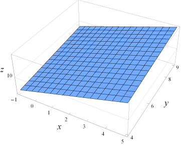
In this problem, the slope of the line segment \(\overline{PQ}\) is computed, first in the direction of the vector \(\overrightarrow{v}\) given in the figure and then in the direction of \(-\overrightarrow{v}\text{.}\) Fill in the table below.
Table 6.7.3.
Direction \(\Delta V\) \(\Delta H\) Slope
\(\vec{v}\)
\(-\vec{v}\)
(b)
Fill the table below based on the graph below.
Table 6.7.4.
Direction \(\Delta V\) \(\Delta H\) Slope
\(\vec{v}\)
\(-\vec{v}\)
(c)
Reflect on the work done in parts (a) and (b).
  1. What is the effect on the slope of a line when the direction \(\vec{v}\) is changed for the opposite direction \(-\vec{v}\text{?}\)
  2. Why must slopes in three dimensions be directed slopes?
  3. How does the slope of a line (in 3D) in direction of a vector \(\vec{v}\) compare with the slope of the same line in direction of vector \(2\vec{v}\) or of vector \(\frac{1}{2}\vec{v}\text{?}\)
  4. A partial derivative of a function of two variables is a slope of a tangent line to the graph of a function in three-dimensional space and hence must be a directed slope. What could be the direction vector (keep in mind that direction vectors only have two coordinates) of a partial derivative with respect to \(x\text{?}\) With respect to \(y\text{?}\)

Activity 6.7.3.

(a)
Let \(f(x,y)=x^2y\text{.}\) Observe that the point \(P=(1,2,2)\) is on the graph of \(f\text{.}\) The figure below represents the tangent plane top the graph of \(f\) at the point \(P=(1,2,2)\text{.}\) The segment \(\overline{PQ}\) is tangent to the graph of \(f\) at the point \(P=(1,2,2)\) in direction of vector \(\langle 3 , 4 \rangle\text{.}\) Its slope in direction of vector \(\langle 3,4 \rangle\) is the directional derivative of \(f\) at the point \((1,2)\) and is denoted \(D_{\langle 3,4\rangle} f (1,2)\text{.}\) In this problem \(D_{\langle 3,4\rangle} f (1,2)\) is computed. Fill the table to aid in your calculation of \(D_{\langle 3,4\rangle} f (1,2)\text{.}\)
Table 6.7.5.
dx dy \(\Delta H\) \(m_x\) \(m_y\) \(\Delta V\) \(D_{\langle 3,4\rangle} f (1,2)\)
_
(b)
Let \(f(x,y)=xy+x\text{.}\) Observe that the point \(P=(2,4,10)\) is on the graph of \(f\text{.}\) The figure below represents the tangent plane top the graph of \(f\) at the point \(P=(2,4,10)\text{.}\) Fill the table to aid in your calculation of \(D_{\langle 3,4\rangle} f (1,2)\text{.}\)
  1. Represent the base point \(P=(2,4,10)\) in the figure below.
  2. Represent the vector \(\angle 3,5\rangle\) in 3D as \(\langle 3,5\rangle\) starting under the base point.
  3. Draw the tangent line to the graph of \(f\) at the point \(P=(2,4,10)\) in the given vector direction.
  4. Fill in the table below to compute the slope \(D_{\langle 3,5\rangle} f (2,4)\)
Table 6.7.6.
dx dy \(\Delta H\) \(m_x\) \(m_y\) \(\Delta V\) \(D_{\langle 3,5\rangle} f (2,4)\)
_
(c)
The following is a table of values for a differentiable two-variable function \(f\text{.}\) Approximate as best you can the value of \(D_{\langle 3,4\rangle} f (1,4)\)
Table 6.7.7.
y=2 y=4 y=4.02 y=6 y=8
x=0 5 7 7.04 10 11
x=1 6 10 10.02 8 9
1.01 6.03 9.96 9.94 9.05 9.10
x=2 10 8 7.80 7 8
x=4 11 8.5 8.01 6 5

Activity 6.7.4.

(a)
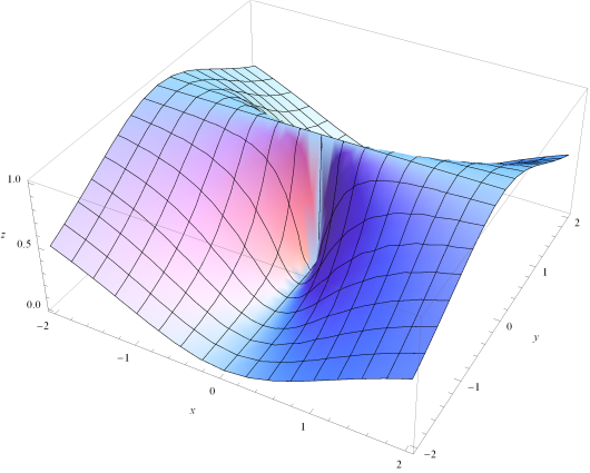
The following is a the graph of \(z=f(x,y)\text{.}\)
  1. On the \(xy\)-plane of the figure below, draw the direction vector \(\langle 1,1\rangle \) starting at the point \((2,-1)\text{.}\)
  2. Draw a piece of the tangent line to the graph of \(f\) at the point \((2,-1,f(2,-1))\) which is in the direction \(\langle 1,1\rangle \text{.}\) The slope of the tangent line in the \(\langle 1,1\rangle \) direction is called the directional derivative of \(f\) at \((2,-1)\) in the \(\langle 1,1\rangle \) direction and is denoted \(D_{\langle 1,1\rangle} f (2,-1)\text{.}\)
  3. Is \(D_{\langle 1,1\rangle} f (2,-1)\) positive, negative, or zero? Justify your answer.
  4. On the \(xy\)-plane of (a new plot of) the figure below, draw the direction vector \(\langle -\frac{1}{2},3\rangle \) starting at the point \((2,-1)\text{.}\)
  5. Draw a piece of the tangent line to the graph of \(f\) at the point \((2,-1,f(2,-1))\) which is in the direction \(\langle -\frac{1}{2},3 \rangle \text{.}\) The slope of the tangent line in the \(\langle -\frac{1}{2},3 \rangle \) direction is called the directional derivative of \(f\) at \((2,-1)\) in the \(\langle -\frac{1}{2},3 \rangle \) direction and is denoted \(D_{\langle -\frac{1}{2},3 \rangle} f (2,-1)\text{.}\)
  6. Is \(D_{\langle -\frac{1}{2},3 \rangle} f (2,-1)\) positive, negative, or zero? Justify your answer.
(b)
Let \(f\) be the function whose graph appears below. For each value of \(t\) the vector \(\langle \cos(t),\sin(t)\rangle \) is a direction vector. The value of \(D(t)=D_{\langle \cos(t),\sin(t)\rangle} f (1,-1)\) is a scalar that measures the rate of change of the function \(f\) in different directions.
  1. What direction (in the xy-plane) is the vector \(\langle \cos(t),\sin(t)\rangle \) in for
    1. \(\displaystyle t=0\)
    2. \(\displaystyle t=\frac{\pi}{2}\)
    3. \(\displaystyle t=\frac{3\pi}{2}\)
    4. \(\displaystyle t=\pi\)
  2. Is the value of \(D(t)=D_{\langle \cos(t),\sin(t)\rangle} f (1,-1)\) positive, negative, or zero for:
    1. \(\displaystyle t=0\)
    2. \(\displaystyle t=\frac{\pi}{2}\)
    3. \(\displaystyle t=\frac{3\pi}{2}\)
    4. \(\displaystyle t=\pi\)
  3. Draw the graph of \(y=D(t)\) for values of \(t\) in the interval \([0,2\pi]\text{.}\) You should think about how the value of \(D(t)\) changes between the values you considered above to help you draw the graph of \(D(t)\text{.}\) Your graph doesn’t have to have exact values but should correctly identify where \(D(t)\) is positive, negative, and zero.
  4. Draw the graph of \(y=G(t)=D_{\langle 1,1 \rangle} f (t,-t)\) for values of \(t\) in the interval \((0,2]\text{.}\) You should probably go through the same process you did above of looking at what \(G(t)\) will be for a few values of \(t\) between 0 and 2, then think about how \(G(t)\) will vary for values in between. The function \(G(t)\) is different than \(D(t)\text{.}\)
(c)
The graph of \(z=f(x,y)\) is as given below. In this problem, use geometric arguments to justify your answers.
  1. Draw the line segment that goes from \((1,-1,f(1,-1))\) to \((2,0,f(2,0))\text{.}\) How does the slope of this line segment in that direction compare (smaller, equal, larger) with the value of \(D_{\langle 1,1 \rangle} f (1,-1)\text{?}\)
  2. How does \(D_{\langle 1,1 \rangle} f (1,-1)\) compare with \(D_{\langle 0.01,0.01 \rangle} f (1,-1)\text{?}\) Justify your answer.
  3. Which is closer to \(D_{\langle 1,1 \rangle} f (1,-1)\text{,}\) the slope of the line segment that goes from \((1,-1,f(1,-1))\) to \((2,0,f(0,2))\) or the slope of the line segment that goes from \((1,-1,f(1,-1))\) to \((1.01,-0.99,f(1.01,-0.99))\text{?}\) Explain your answer.