Create a vector valued function representing a section or contour for a multivariable function
Understand the relationship between a contour plot and a multivariable function
Subsection6.3.1Sections on Graphs of Multivariable Functions
Activity6.3.1.Using Sections to Draw MVF graphs.
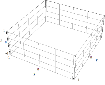
Let \(f(x,y)=yx^2\) with domain restricted to \(\{(x,y)|-1\geq x \geq 1, -1\geq y \geq 1\}\text{.}\) We will use the steps below to try to make a good plot of \(z=f(x,y)\text{.}\)
(a)
Draw the section corresponding to \(y=-1\) on the image provided above.
(b)
Draw the section corresponding to \(y=1\) on the image provided above.
(c)
Draw the section corresponding to \(x=-1\) on the image provided above.
(d)
Draw the section corresponding to \(x=1\) on the image provided above.
(e)
Use other sections as appropriate to complete the graph of \(z=f(x,y)\text{.}\)
Subsection6.3.2Contours and Level Curves
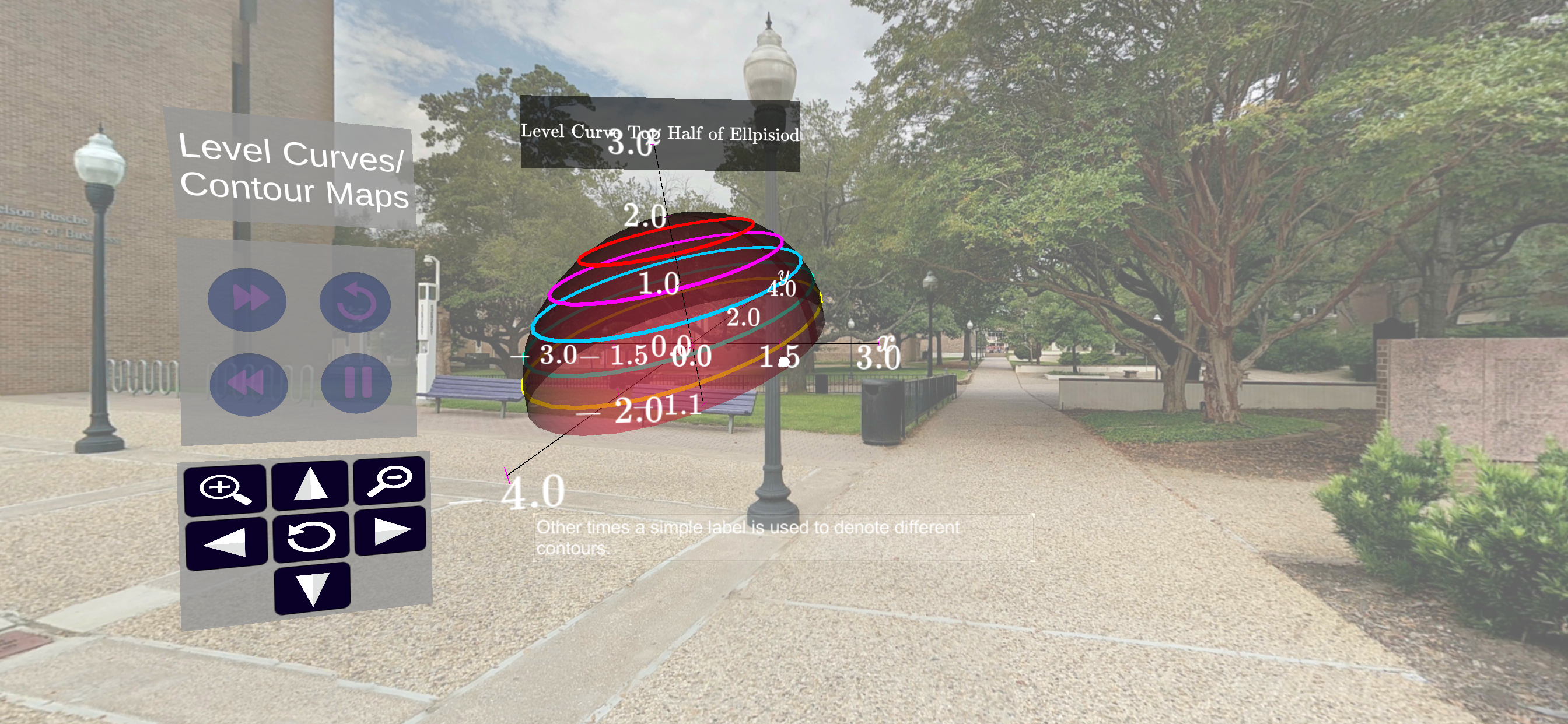
Figure6.3.1.A screenshot from the lesson on level curves and contours of multivariable functions.
We have explored means for studying multivariable functions using contour plots. To find a specific contour for a function \(z=f(x,y)\) we substitute a value \(c\) for \(z\) and find the resulting two dimensional graph of
In this way, the value of \(c\) can be thought of as the elevation we are interested index and the graph of \(c=f(x,y)\) represents multivariable surface at that elevation. Often times it is useful to describe these graphs with one or more parametric equations.
Give enough values to either \(x\) or \(y\) until you can imagine how the graph of \(z=f(x,y)\) looks in space. Draw the graph as carefully as you can and include a verbal description for your surface.
\(\displaystyle f(x,y)=x-y^2\)
\(\displaystyle f(x,y)=(x+y)^2\)
\(\displaystyle f(x,y)=\sqrt{x-y}\)
\(\displaystyle f(x,y)=\sqrt{y-x^2}\)
(b)
Draw a contour diagram for the function \(z=f(x,y)\) as carefully as you can and verify that your diagram is consistent with the graph you drew in the previous part. You must draw enough contours so that the behavior of the function in all of its domain may be deduced. Show all your work.
\(\displaystyle f(x,y)=x-y^2\)
\(\displaystyle f(x,y)=(x+y)^2\)
\(\displaystyle f(x,y)=\sqrt{x-y}\)
\(\displaystyle f(x,y)=\sqrt{y-x^2}\)
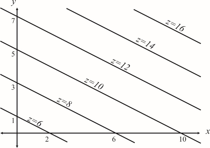
Activity6.3.4.
The following is a contour diagram of a plane.
(a)
Find \(m_x\text{.}\) (Remember that the plane is in 3D and that therefore both \(x\) and \(y\) refer to “horizontal”, while “vertical” refers to \(z\)).
(b)
Find \(m_y\text{.}\) (Remember that the plane is in 3D and that therefore both \(x\) and \(y\) refer to “horizontal”, while “vertical” refers to \(z\)).
(c)
Express vertical change \(dz\) as a function of the horizontal change in the \(x\) direction and the horizontal change in the \(y\) direction (that is, in terms of \(dx\) and \(dy\)).
Exercises6.3.3Exercises
For the following sketch a contour map of the surface using level curves for the given \(c\)-values.