To understand how a parametric equation can be used to specify and generate a curve.
To learn how to graph a line using parametric equations.
To learn how to graph transformations of a circle using parametric equations.
In this section, we will explore parametric curves, thier definitions, and how to graph a system of parametric equations.
Subsection1.1.1Curves
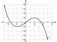
Throughout calculus you have studied functions and their corresponding graphs. Typically you were given a function of the form \(y=f(x)\) and were asked to construct or identify a corresponding graph, such as
A more powerful means of constructing curves in two dimensional space can be found through the use of parametric equations. A parametric equation is of the form
For Activity 1.1.1, we will examine the parametric equations given by \(x(t)=t-2\) and \(y(t)=4-t^2\) and the corresponding graph.
1.
In the table given on the left of Figure 1.1.1, you should enter at least seven values into the \(t\) column. How are the numbers you are entering relating to the points being graphed?
Figure1.1.1.A Desmos Example for use with Activity 1.1.1
Hint.
Use both positive and negative numbers for \(t\text{,}\) such as \(-3,-2,-1,0,1,2,3\text{.}\) You should also consider values that are not integers.
2.
Explain what shape you think the points given by these parametric equations will draw. Be sure to note any particular features of that graph that you can identify from examining your set of points in Figure 1.1.1.
3.
You should draw your seven points by hand on a set of axes and label each point with its corresponding \(t\) value. If you think of \(t\) as time, the value of \(t\) shows you how an object would move along this curve over time. This idea is often referred to as orientation.
Sometimes we can revert back to equations in terms of \(x\) and \(y\) by eliminating the parameter\(t\text{.}\) Notice that for the equation above we have
Substitute the result for \(t\) from the last part into the equation \(y=4-t^2\) to get an equation in terms of just \(x\) and \(y\text{.}\) Be sure to write down your equation and specify what shape the graph of this equation will have.
(c)
Graph the equation in \(x\) and \(y\) from the previous part using the input box that starts with \(y=\) (in Figure 1.1.1). Does your equation in \(x\) and \(y\) give you the same picture as the parametric equations? Be sure to explain any difference between your earlier prediction and what you see in the \(xy\)-graph.
Activity1.1.1.Parametric Equations and Lines in 2D.
(a)
Draw the line through the points \((1,2)\) and \((5,4)\text{.}\) To go from \((1,2)\) to \((5,4)\) how far would you have to walk in the \(x\) direction? How far in the \(y\) direction?
Notice that when you plug in \(t=0\) you are at the starting point \((1,2)\text{.}\) What needs to be placed in each \(\underline{\hspace{0.2in}}\) to have an output point of \((5,4)\) when \(t=1\text{?}\)
(c)
Explain how the slope of the line relates to the parametric equations you found in the previous part?
(d)
In Figure 1.1.3, the line \(y=3x+4\) is plotted. Give parametric equations for the line \(y=3x+4\) and graph your parametric equations to make sure the parametric equations represent the given line. Explain how you got your parametric equations.
Try to either find two points on the line \(y=3x+4\) or use a point and the slope.
(e)
Is their only one set of parametric equations for \(y=3x+4\) or can you come up with other parametric equations for \(y=3x+4\text{?}\) Explain your reasoning.
Subsection1.1.2Circles
From basic trigonometry you should remember the Pythagorean identity
Consider both equations for the unit circle as plotted in the Desmos Interactive below. As \(t\) starts at 0 and goes to \(t=2\pi\text{,}\) describe the way the parametric equation traverses the circle. Where do we "start"? In what direction do we move along the circle (clockwise or counterclockwise)?
(b)
Change both the parametric equations and the equation in \(x\) and \(y\) so that the circle has a radius of 3.
(c)
Change both the parametric equations and the equation in \(x\) and \(y\) so that the circle has a center of \((-1,2)\)